
Property tax revenue is one of the most stable and significant funding streams for municipal governments, but “stable” doesn’t mean easy to predict. Assessed values fluctuate with the housing market, shift dramatically after reappraisal cycles, and interact in complex ways with macroeconomic conditions. At the City of Seattle’s Office of Economic and Revenue Forecasts (OERF), I’ve been building a parcel-level machine learning pipeline to forecast assessed values (AV) through 2031, replacing a simpler aggregate-extrapolation approach with a system that learns from the full cross-sectional and temporal structure of the tax roll.
This one is a check-in after the April 2026 forecast cycle, with three major changes worth documenting: macroeconomic and housing-market conditioning, a three-track architecture covering Residential, Condo, and Commercial separately, and a sequential year-by-year forecast run under baseline, optimistic, and pessimistic scenarios. Everything is anchored to the $306.5B certified AV base for tax year 2026.
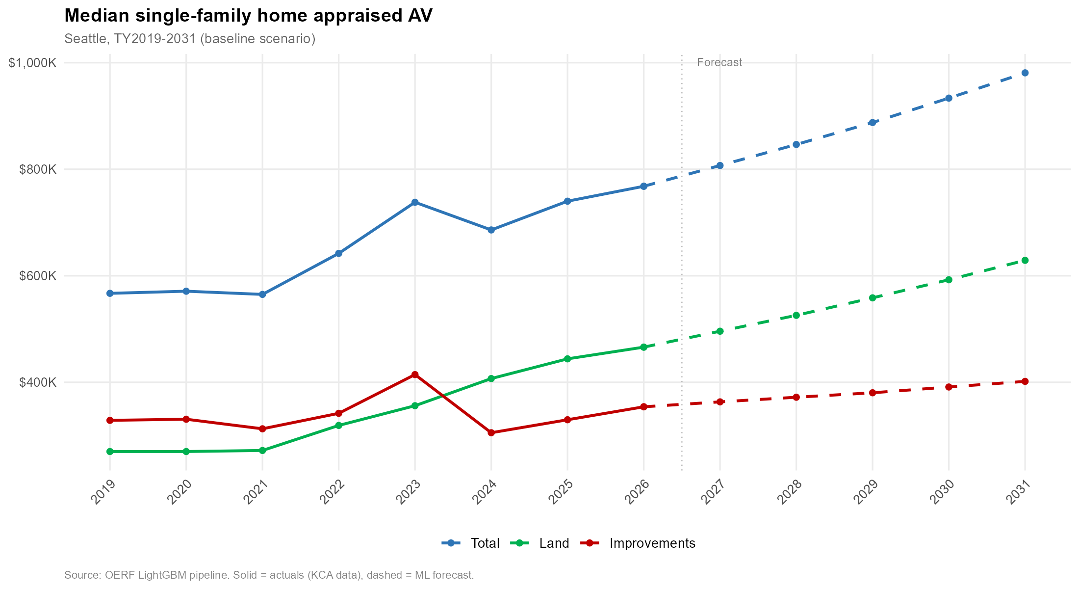
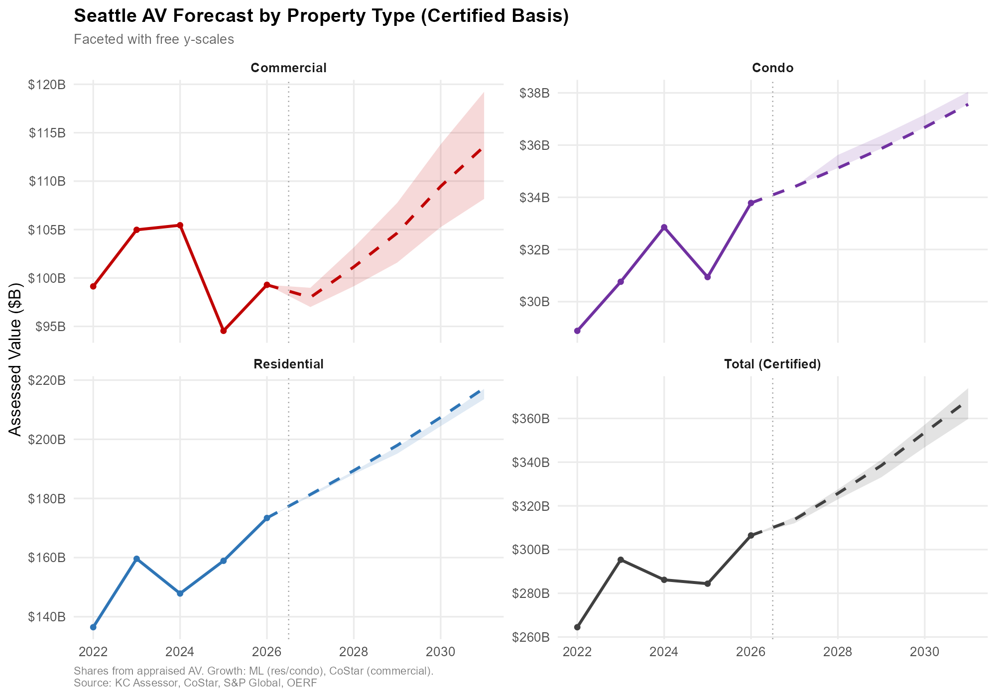 Historical (solid) and forecast (dashed), separate scales. Shaded areas = optimistic/pessimistic range. Source: KC Assessor, CoStar, S&P Global, OERF.
Recap: The Residential Prototype
The starting point was a LightGBM parcel-level model for residential property (prop_type R, roughly 179K parcels), trained on King County Assessor panel data from 2006 to 2026. Features were parcel characteristics: square footage, lot size, year built, location, view score, and so on. The model produces point-in-time AV predictions per parcel, which aggregate up to citywide totals.
Why LightGBM
LightGBM is a decision tree ensemble, similar in spirit to random forest but with three design choices that make it both faster and more accurate in this setting:
- Gradients. Parcels with large residuals are weighted more heavily in subsequent sampling, so harder-to-predict parcels drive the tree splits.
- Boosting. Trees are grown sequentially, each one correcting the errors of its predecessors.
- Histogram binning. Continuous features are bucketed, which shrinks the search space for splits and speeds up training dramatically.
For a panel with hundreds of thousands of parcels and twenty years of history, those three properties matter.
The retrofitted panel
The “retrofitting” part of the prototype refers to filling in parcel-year cells where the Assessor’s historical extracts are incomplete. A parcel might have observed land and improvement AVs in 2021, 2024, and 2025, but nothing for 2022 or 2023. The first model pass predicts AVs for those missing historical cells using surrounding observed values and parcel characteristics, producing a dense panel that can then be used for forward forecasting.
A simplified illustration, before and after retrofitting:
| Parcel ID | Land AV | Imp. AV | Tax Year | Lot Sqft | Imp. Sqft | View |
|---|---|---|---|---|---|---|
| 1000111111 | $500,000 | $500,000 | 2025 | 2000 | 1500 | 5 |
| 1000111111 | $500,000 | $500,000 | 2024 | 2000 | 1500 | 5 |
| 1000111111 | N/A | N/A | 2023 | 2000 | 1250 | 3 |
| 1000111111 | N/A | N/A | 2022 | 2000 | 1250 | 3 |
| 1000111111 | $400,000 | $350,000 | 2021 | 2000 | 1100 | 2 |
After retrofitting, the missing 2022 and 2023 rows are filled in with model-based estimates consistent with surrounding vintages and parcel attributes.
What’s New: Integrating Macro and Sales Data
The prototype relied almost entirely on parcel-level attributes. The updated pipeline adds a second family of features that vary over time and across scenarios:
- Macroeconomic inputs from OERF’s regional forecasting model: employment levels and YoY growth by sector, income growth, housing permits, the Case-Shiller home price index, CPI, and related series.
- Housing market inputs from NWMLS: median sale prices, closed sales volume, and active listings, at both Seattle and King County levels and across multiple lags.
Crucially, these time-varying features vary by scenario. The baseline, optimistic, and pessimistic macro paths feed different feature values into the same trained model, which is what differentiates the three forecast trajectories. The parcel characteristics stay fixed; the economic and market context is what varies.
The extended panel looks like this:
| Parcel ID | Land AV | Imp. AV | Year | Lot Sqft | Imp. Sqft | View | Type | NWMLS Med | OERF Emp |
|---|---|---|---|---|---|---|---|---|---|
| 1000111111 | N/A | N/A | 2031 | 2000 | 1100 | 5 | Res | $1.5M | 1200 |
| 1000111111 | N/A | N/A | 2029 | 2000 | 1100 | 5 | Res | $1.4M | 1200 |
| 1000111111 | N/A | N/A | 2028 | 2000 | 1100 | 5 | Res | $1.3M | 1100 |
| 1000111111 | N/A | N/A | 2027 | 2000 | 1100 | 5 | Res | $1.2M | 1100 |
| 1000111111 | $500,000 | $500,000 | 2026 | 2000 | 1100 | 5 | Res | $1.1M | 1000 |
Three-Track Architecture
The single biggest structural change is that the pipeline now runs three separate tracks: Residential, Condo, and Commercial. Each track has its own model training, its own feature engineering, and its own forecast logic.
The rationale is that the Assessor uses genuinely different valuation methodologies for these property types. Residential and condo valuations lean heavily on comparable sales, which is a pattern ML learns well from parcel-level panel data. Commercial properties, especially investment-grade ones, are predominantly assessed via income capitalization and cap rates applied to net operating income. That’s a different data-generating process, and forcing it through a single model gives up information in both directions.
Condo track
Condos get modeled separately from single-family homes. The parcel universe is smaller and the feature importance profile is different: building-level attributes (complex condition, effective year built, number of bedrooms, effective unit square footage, and view share) matter more relative to lot-based features, which makes sense since a condo unit doesn’t have a dedicated lot. Parcel-level predictions are noisier, but aggregation to citywide totals stabilizes them. Validation was against the Assessor’s condo area reports.
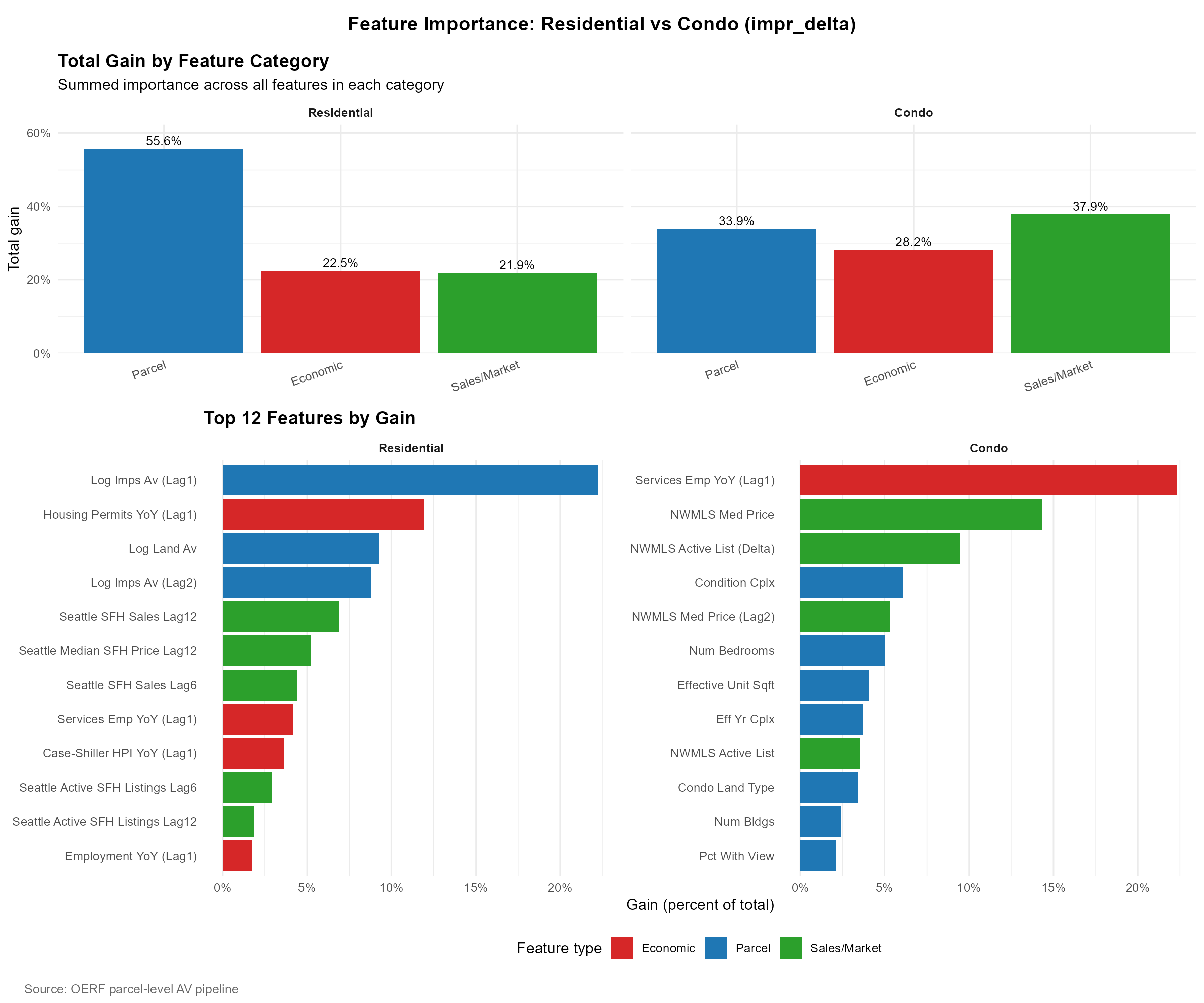 Source: OERF ML Model.
The feature importance profile between residential and condo is a useful contrast. For residential, parcel characteristics dominate total gain (55.6%), with economic (22.5%) and sales/market (21.9%) features playing smaller but still substantial roles. The top individual feature is the first lag of log improvements AV, followed by housing permits growth and log land AV. For condos, the mix is much more balanced: sales/market features actually lead (37.9%), then parcel (33.9%), then economic (28.2%). The single most important condo feature is the first lag of services employment YoY growth, followed by NWMLS median price and the year-over-year change in active listings.
Commercial track
The commercial track went a different direction. I initially built a parcel-level ML commercial panel, but the output had a 134% aggregate growth rate anomaly that couldn’t be reconciled with any plausible trajectory. The root cause is the income-capitalization issue above: cap rates and net operating income are the primary signals the Assessor actually uses, and the ML panel didn’t have direct access to either.
Rather than force it, the decision was to bypass ML for commercial in this forecast cycle and fall back to the prior model that applies growth rates sourced from CoStar. The commercial forecast is broken out into seven groups: Apartment, Major Office, Industrial, Hospitality, Medical, Retail, and Other, each with its own growth assumption anchored in the CoStar feed.
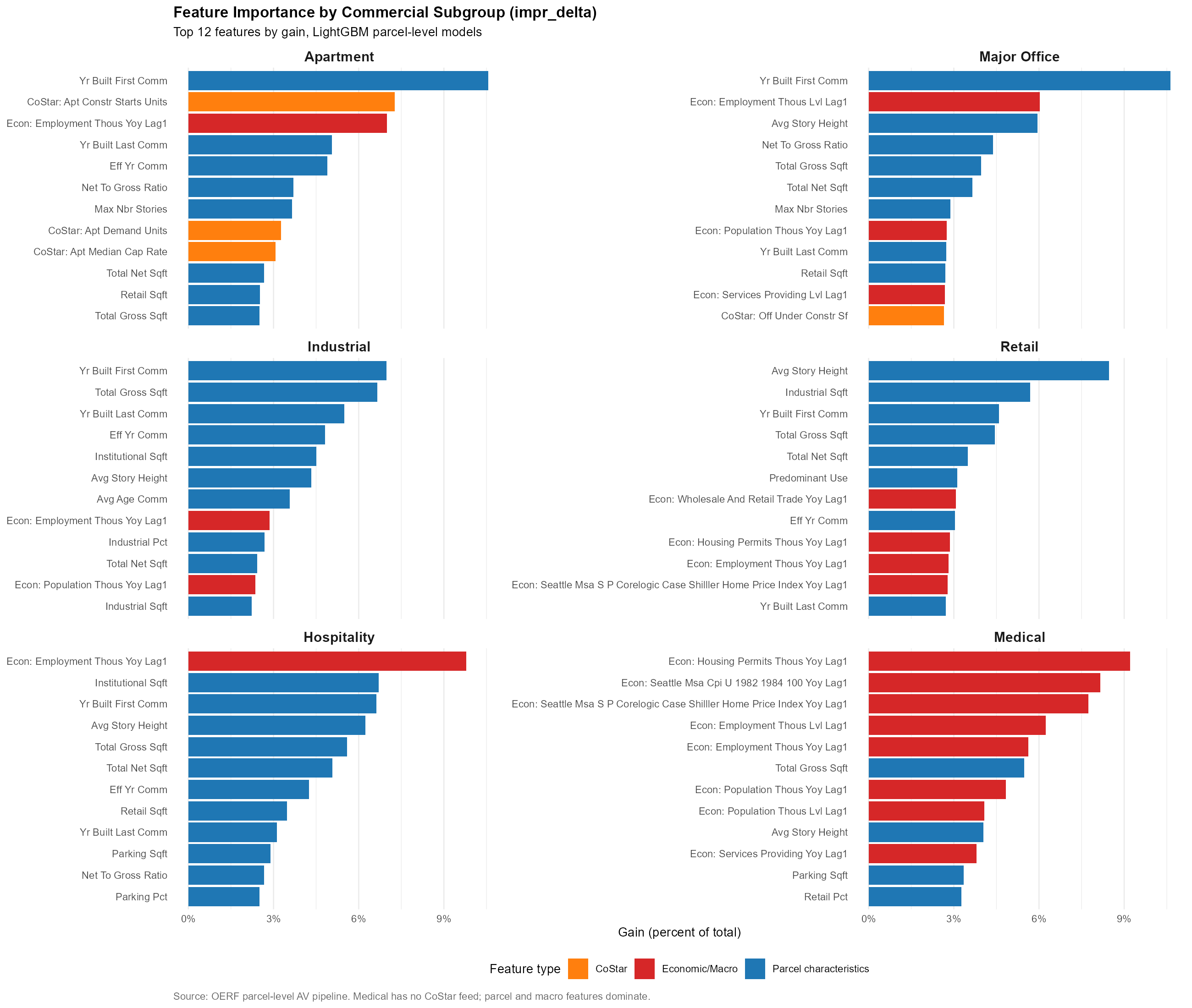 Source: OERF ML Model, WIP.
That said, the exploratory ML work on commercial produced useful feature-importance diagnostics by subgroup. For Apartment, the first lag of services employment growth, first lag of employment levels, and several CoStar supply-side indicators (apartment construction starts, apartment demand units, median cap rate) rank near the top. For Major Office, building characteristics (year built, story height, net-to-gross ratio) dominate, with employment levels as the leading macro. Hospitality is the most macro-sensitive of the commercial subgroups, employment YoY growth is by far the single most important feature. Medical is also heavily macro-driven, with housing permits, CPI, and Case-Shiller all in the top five. That profile is what motivates the next-step plan to build separate ML models per commercial group rather than a single pooled commercial model.
Sequential Year-by-Year Forecast
The forecast is not a single forward pass to 2031. It’s a sequential simulation where each year’s predictions become features for the next year.
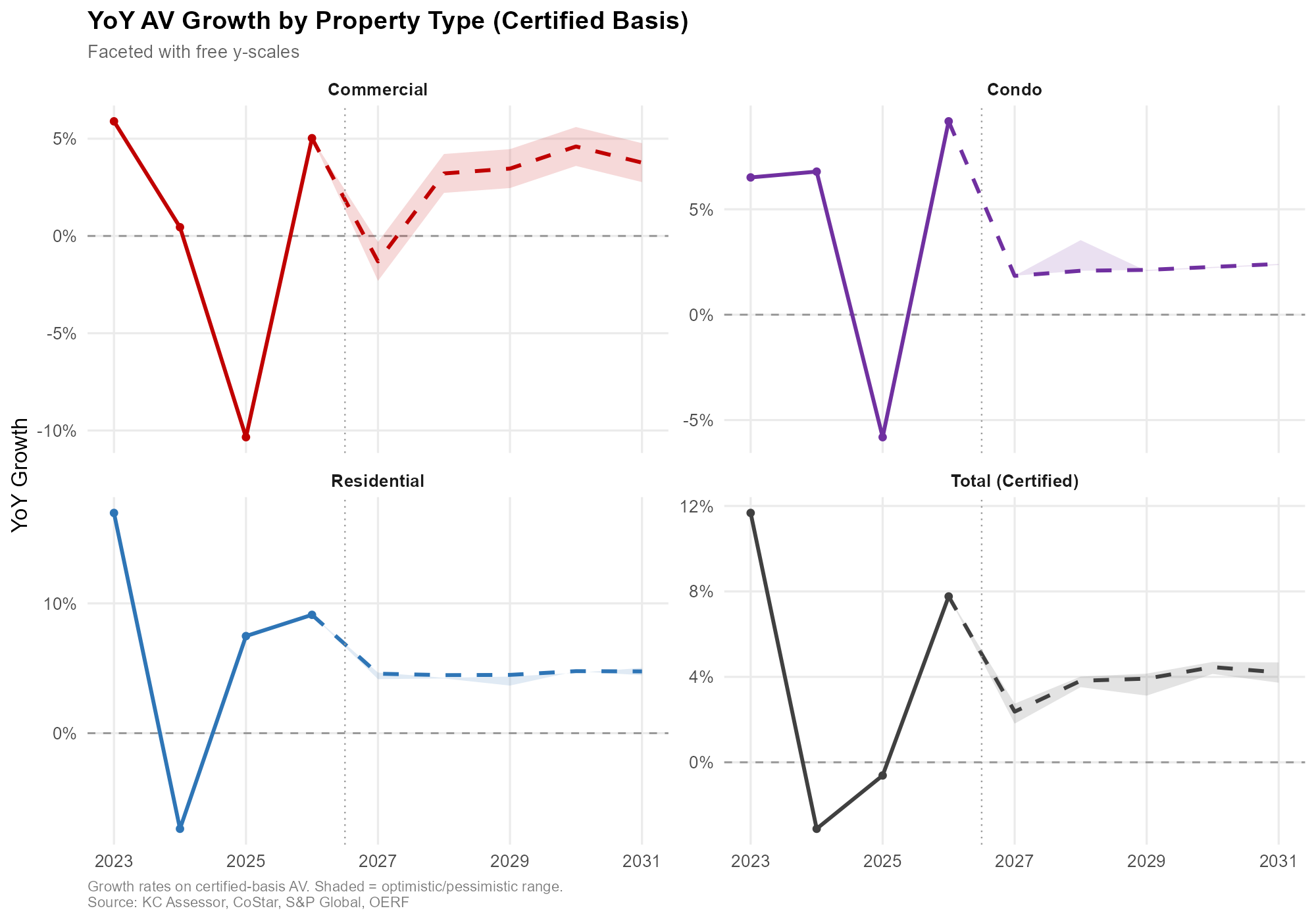
 Historical (solid) and forecast (dashed). Shaded areas = optimistic/pessimistic range. Source: KC Assessor, CoStar, S&P Global, OERF.
The loop is:
- Train the model on the historical panel, 2006 through 2025 observed AVs.
- Predict 2026 AV per parcel using 2025 actuals plus 2026 macro inputs.
- Append 2026 predictions to the panel. Predict 2027 using predicted 2026 AV plus 2027 macro inputs.
- Repeat year by year through 2031.
- Output:
panel_tbl_2006_2031_forecast_{scenario}_{track}.rds.
This structure captures path dependency. A parcel that appreciates in 2026 starts from a higher base in 2027, and a parcel that undershoots doesn’t automatically snap back. The sequential approach also lets mean-reverting dynamics emerge naturally. Parcels with anomalously large predicted jumps in one year tend to revert partially the next, consistent with how the Assessor’s smoothing behaves in practice.
The same loop runs three times per track, once for each scenario (baseline, optimistic, pessimistic), with different macro and NWMLS input vectors.
Schematically, the forecasted panel fills in one year at a time:
| Parcel ID | Land AV | Imp. AV | Year | … | NWMLS | OERF |
|---|---|---|---|---|---|---|
| 1000111111 | $650,000 | $600,000 | 2031 | … | $1.5M | 1200 |
| 1000111111 | $600,000 | $600,000 | 2029 | … | $1.4M | 1200 |
| 1000111111 | $600,000 | $550,000 | 2028 | … | $1.3M | 1100 |
| 1000111111 | $550,000 | $550,000 | 2027 | … | $1.2M | 1100 |
| 1000111111 | $500,000 | $500,000 | 2026 | … | $1.1M | 1000 |
Anchoring to the Certified Base
All forecasts are anchored to the $306.5B certified AV for tax year 2026. A reconciliation step ensures that parcel-level predictions for the base year sum to the known certified totals by property type before projecting forward. Growth rates from 2026 onward are applied to the certified base, which keeps the forecast grounded in the Assessor’s official starting point rather than drifting based on ML-estimated 2026 levels.
New construction AV is handled separately, using levy worksheet history back to 2007 rather than the ML panel. That’s partly a data issue (the retrofitted panel isn’t the right source for NC) and partly a concept issue. NC is additive on top of the existing roll and deserves its own treatment.
Results Summary
Model-level diagnostics on the held-out validation split:
| Track | Target | RMSE (log) | MAE (log) | MAPE | WAPE |
|---|---|---|---|---|---|
| Residential | Land | 0.128 | 0.057 | 6.1% | 5.7% |
| Residential | Improvements | 0.629 | 0.232 | 28.7% | 17.0% |
| Condo | Land | 0.073 | 0.061 | 6.0% | 6.1% |
| Condo | Improvements | 0.206 | 0.129 | 14.1% | 12.5% |
| Commercial | Land | 0.151 | 0.066 | 10.6% | 6.7% |
| Commercial | Improvements | 1.320 | 0.499 | 137.0% | 27.2% |
A few things to read out of this table. Land is easier to predict than improvements across all three tracks, which is consistent with land values being smoother and more spatially determined. Condo improvements are the best-predicted improvement series (WAPE 12.5%), which is a pleasant surprise and suggests that once you have the right building-level features, condo value trajectories are reasonably tractable. Commercial improvements is where the wheels come off: WAPE of 27% and MAPE of 137%, which is the numerical fingerprint of the income-capitalization mismatch. That result is the main reason the commercial track falls back to CoStar growth rates rather than ML for this forecast cycle.
How the Metrics Were Produced: Rolling-Origin Cross-Validation
Random k-fold cross-validation is the wrong design for a panel like this. Parcels in 2025 are not independent draws from the same distribution as parcels in 2010, and the actual forecasting task is to predict future years using past years. Random folds let information from 2024 leak into a model that is then evaluated on 2015, which flatters the metrics in a way that has nothing to do with how the model performs in production.
Instead, every track uses rolling-origin CV cut by tax year. The folding function (make_rolling_year_folds() in 00_init.R) picks five chronological cutpoint years evenly spaced across the panel. For each cutpoint, the training set is every parcel-year with tax_yr <= cutpoint, and the validation set is every parcel-year with tax_yr > cutpoint. Training expands forward with each fold; validation is the entire future tail of the panel relative to the cutpoint.
For the 2006–2025 historical panel with five folds and min_train_yrs = 3, the cutpoints land at 2008, 2012, 2016, 2020, and 2024:
| Fold | Train (years ≤ cutpoint) | Validate (years > cutpoint) |
|---|---|---|
| 1 | 2006–2008 | 2009–2025 |
| 2 | 2006–2012 | 2013–2025 |
| 3 | 2006–2016 | 2017–2025 |
| 4 | 2006–2020 | 2021–2025 |
| 5 | 2006–2024 | 2025 |
A few things this design is doing deliberately. Every fold respects the arrow of time: the model never sees future years during training, which matches the production forecasting task. Training grows with each fold, so later folds have more history to learn from, which mirrors how the model will actually be refit in production over time. And validation on the full future tail (rather than just the next year) stress-tests the model across multiple forecast horizons within a single fold. Fold 1 is a hard test: train on only three years, then predict seventeen years of AVs. Fold 5 is an easy test: train on almost everything, then predict one year. The metrics in the table average across all five, so they reflect performance across a range of training-history depths and forecast horizons rather than a single favorable configuration.
One trade-off to flag honestly. Because early folds have short training windows and long validation tails, their per-fold RMSE is higher than later folds. The aggregate metric is an unweighted average across folds, which is a conservative choice: it weights the hard folds the same as the easy ones, so the reported numbers are closer to worst-case than best-case. A production refit on the full 2006–2025 panel, which is what the sequential forecast actually uses, should perform better than the CV numbers suggest.
Layered on top of the CV, 05_eval_holdout_2025.R runs a dedicated backtest: fit the full pipeline on 2006–2024 and predict 2025, then compare predicted aggregate AV against the certified 2025 roll. This is the cleanest out-of-sample check available, because 2025 is a year the model has not seen in training or CV, and the certified roll is ground truth.
The commercial improvements WAPE of 27% is a real out-of-sample number across multiple horizons, not an artifact of a leaky split. That is part of why the decision to fall back to CoStar for commercial is a judgment the validation actually supports, rather than a convenient retreat.
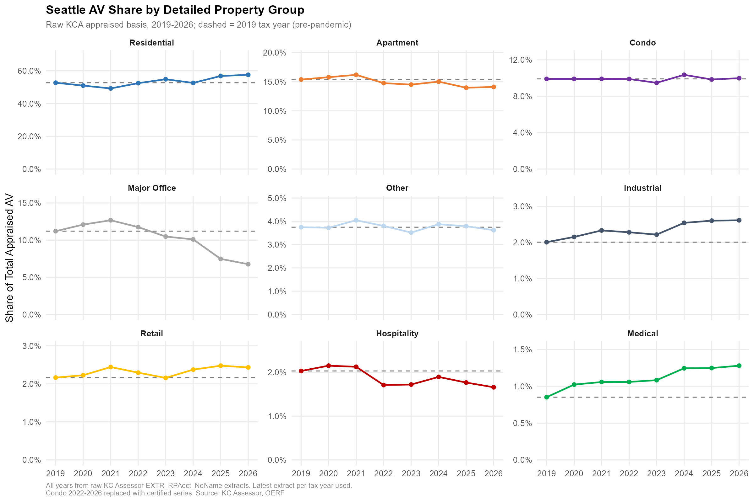
Seattle AV Shares: 2019 vs. 2026
Some context for where the $306.5B base is coming from and how composition has shifted in the last seven years:
| Group | 2019 ($B) | 2026 ($B) | % Change | 2019 Share | 2026 Share | Δ Share |
|---|---|---|---|---|---|---|
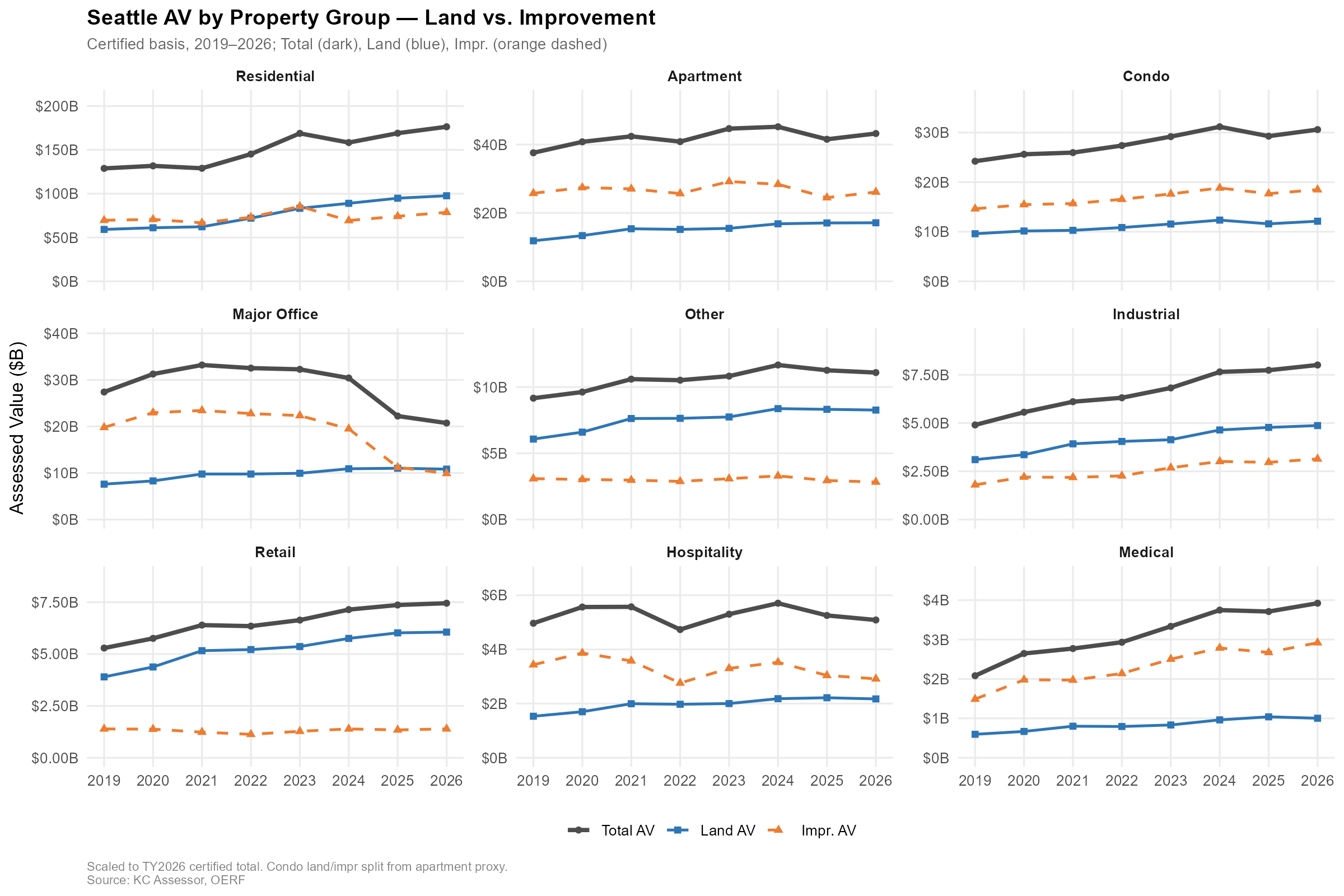
| Residential | 128.9 | 176.3 | 36.9% | 52.7% | 57.5% | +4.8 pp |
| Apartment | 37.6 | 43.2 | 15.0% | 15.4% | 14.1% | –1.3 pp |
| Condo | 24.2 | 30.6 | 26.4% | 9.9% | 10.0% | +0.1 pp |
| Office | 27.4 | 20.7 | –24.3% | 11.2% | 6.8% | –4.4 pp |
| Retail | 5.3 | 7.5 | 40.9% | 2.2% | 2.4% | +0.3 pp |
| Hospitality | 5.0 | 5.1 | 2.4% | 2.0% | 1.7% | –0.4 pp |
| Industrial | 4.9 | 8.0 | 63.4% | 2.0% | 2.6% | +0.6 pp |
| Medical | 2.1 | 3.9 | 88.4% | 0.9% | 1.3% | +0.4 pp |
| Other | 9.2 | 11.1 | 21.1% | 3.7% | 3.6% | –0.1 pp |
| Total | 244.5 | 306.5 | 25.4% |
The residential rise and the office collapse are the two headline shifts. Residential grew 36.9% in dollars and picked up nearly five percentage points of share. Office lost a quarter of its AV outright and gave up 4.4 points of share. This is the story covered in a separate post on Seattle’s biggest office buildings losing half their AV in three years. Industrial and medical are the quiet growth stories, each up more than 60% in dollars, though from smaller bases.
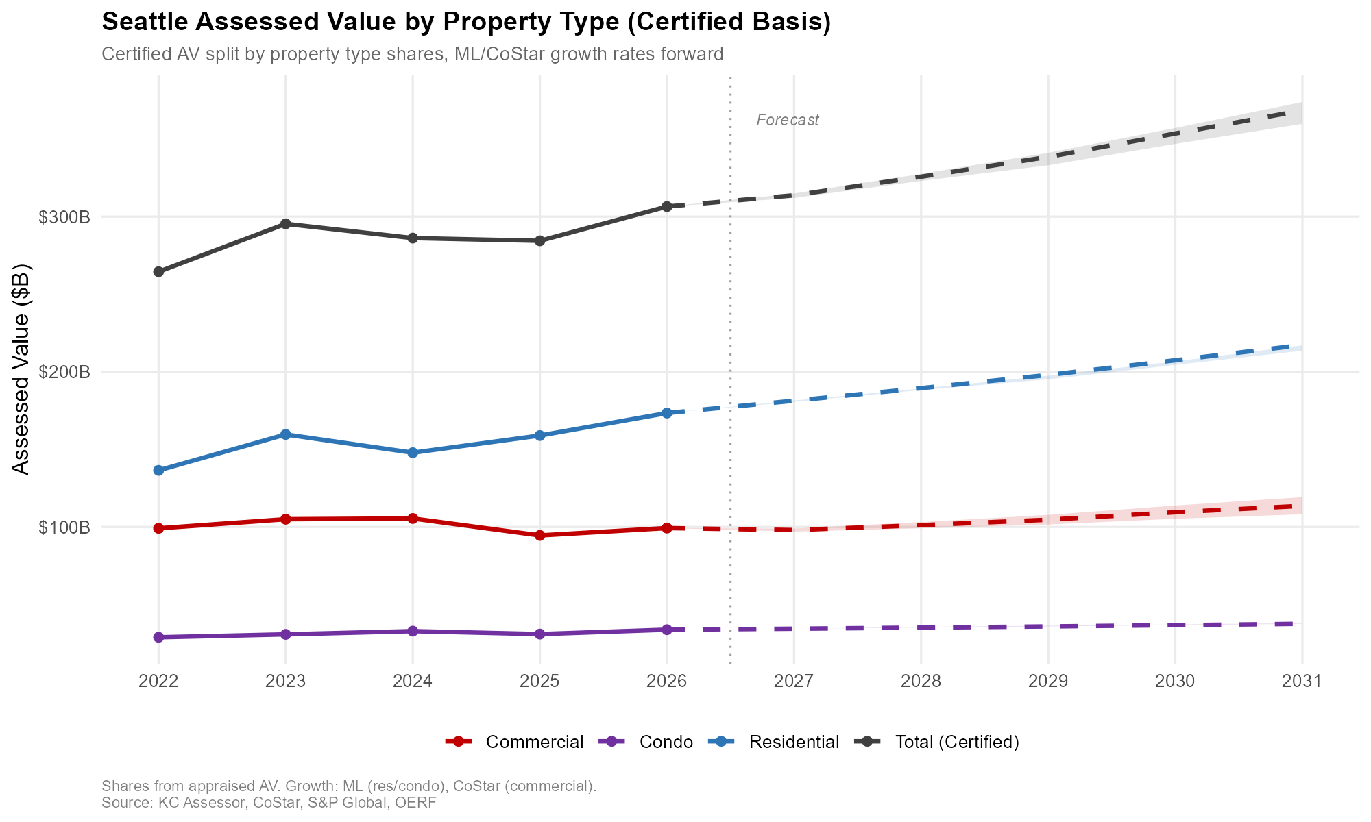
 Historical (solid) and forecast (dashed), separate scales. Shaded areas = optimistic/pessimistic range. Source: KC Assessor, CoStar, S&P Global, OERF.
 Historical (solid) and forecast (dashed). Source: KC Assessor, CoStar, S&P Global, OERF.
Lessons Learned
A few things have held up across this iteration:
Parcel-level ML works where the valuation logic is sales-driven. Residential and condo are comparable-sales regimes, and the models do well there. Commercial is primarily income-capitalization, and parcel features plus macro features don’t substitute for cap rate and NOI data. The honest answer is to use a different tool for commercial, at least until the ML panel can incorporate income-side features.
Data engineering was at least half the work. Parcel ID format mismatches (dashes vs. no dashes causing empty training joins), data.table and tidyselect type conflicts, vintage accuracy in the retrofitted panel, memory management during chunked prediction — these ate more time than model tuning did. None of it is visible in the output, but all of it had to be right for the output to mean anything.
Anchoring matters more than raw model accuracy. Reconciling to the certified $306.5B base before projecting forward is what makes the forecast defensible to stakeholders. A model that’s accurate in log space but drifts from the known certified level is less useful than one that’s anchored and then applies plausible growth rates.
Next Steps
The main item on the roadmap is refining the commercial approach. Rather than a single pooled commercial model, the plan is separate ML models for separate commercial groups (Major Office, Apartment, Industrial, etc.), each with subgroup-specific features. The feature-importance diagnostics already show that the right features differ substantially across subgroups (Hospitality is macro-dominated, Major Office is building-characteristic-dominated, Medical leans on housing permits and home price indices), which is a strong signal that subgroup models will outperform a pooled one.
 Source: King County Assessors
Beyond that, the near-term roadmap is to fold income-side features (cap rates, NOI proxies from CoStar) into the commercial ML panel, which should address the 134% growth anomaly directly rather than working around it. And further out, the sequential scenario framework is a natural fit for richer scenario analysis tied to OERF’s broader regional model.
The code for this pipeline is here. If you’re working on similar problems in municipal finance or property tax forecasting, feel free to reach out.
Start the conversation